Contractional fault-related folding: Implications for localized fracturing

Introduction

The purpose of this section is to illustrate how contractional folding produces structural domains with different deformation histories. These deformation histories control fracture development. The general concepts of structural domains and structurally-controlled fracturing are independent of any structural model. The primary discussion focuses on constant bed length and constant bed thickness folding. However, unlike extensional fault bend folding, there are different types of contractional fault-related folding that produce different fold geometries and have very different implications for fracture development. Fault propagation and trishear folding are mentioned in short sections after the discussion of fault bend folding with constant bed length and thickness. This page does not cover other geometries such as area balanced cross sections. Contractional fold geometries can be complex. If you want to understand how fractures are distributed around a fold, then you require a sound understanding of how the fold developed.

Fault bend folding with constant bed length and thickness

The discussion in this section is based on a conceptual model of fault-bend folding described in: J. Suppe, 1983, Geometry and kinematics of fault-bend folding: American Journal of Science, v. 283, p. 684–721.

Constraints and assumptions of the model: bed length is conserved; bed thickness is conserved; flexural-slip deformation only (simple-shear deformation by slip along bedding planes combined with flexure of the strata — what happens when you bend a deck of cards); no out-of-plane movement.

Initial state

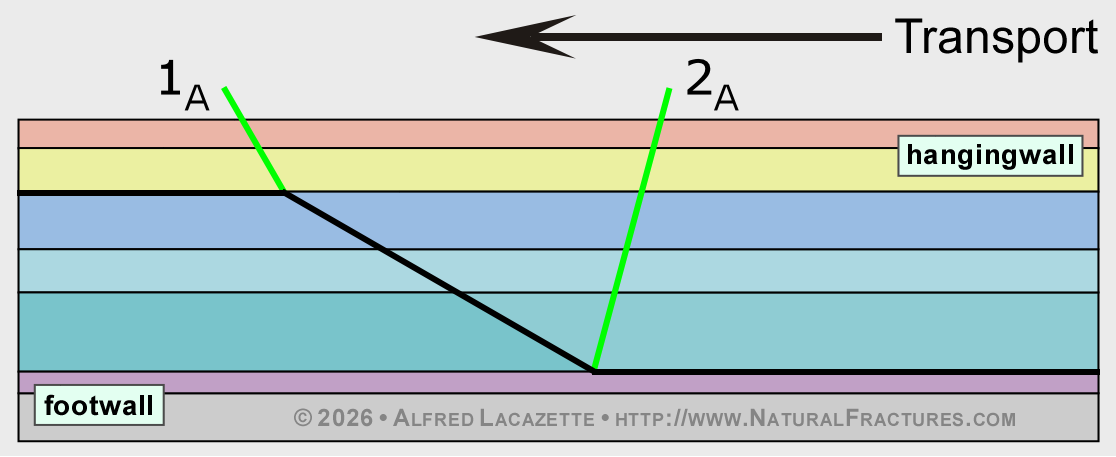
Thrust faults typically run parallel to bedding in weak horizons (such as shales) and then ramp steeply through competent stratigraphic packages (such as carbonates) until they encounter another weak horizon. Folding begins at the active axial planes as soon as the hangingwall block begins moving.

Figure 1. Figure 1. Thrust faults typically run parallel to bedding in weak horizons (such as shales) and then ramp steeply through competent stratigraphic packages (such as carbonates) until they encounter another weak horizon, as shown in this figure. Folding begins at the active axial planes (green) as soon as the hangingwall block begins moving.

Folding processes and strain

As flat-lying strata are pushed onto the ramp they fold to match the ramp angle at axial plane 2. At the top of the ramp the strata must collapse along axial plane 1 to fill the void. The type of strain required by this model is termed simple shear. The type and amount of shear at each active axial plane can be calculated directly from the model. Some slip is consumed by folding.

Figure 2. Folding process and strain at the ramp.

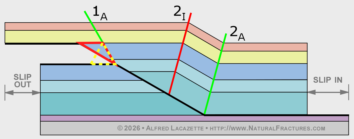
The folding process at the top of the ramp is less obvious. Clearly, strata above the ramp cut-off do not fold as long as they are above the ramp. At the top of the ramp the strata must collapse along axial plane 1 to fill the void. Strata within the red triangle fold to form the dashed yellow triangle, which has the same area as the red one. Substantial slip is consumed by this folding process.

Strain due to folding. Folding requires shear strain of the individual strata that lie between slip surfaces as well as of the entire stratigraphic column. The type of strain required by this model is termed simple shear. When you push a deck of cards so that it slides to form a stack with slanted edges, you have deformed the deck of cards by simple shear. The type and amount of shear at each active axial plane can be calculated directly from the model. Unfortunately, this model does not accurately represent all aspects of natural folding. This model works well for analyzing large structures because the entire stack of strata does appear to deform by flexural-slip in nature. However, individual strata between slip-surfaces do not deform internally by simple shear so strain predictions from this model are not a good predictor of fracture system properties. The actual strain mechanisms of individual strata are beyond the scope of this page. A page on the subject will be added to this website, eventually.

Anticlinal growth stage

Active axial planes (green) do not move because they are pinned to the fault bends. Inactive axial planes (red) move with the hangingwall block. Rocks that have been folded are more likely to be fractured (gray). Most of the fault slip coming into the structure is consumed by anticlinal growth. Consequently, the slip-rate of the fault on the upper flat (above/in front of the ramp) is substantially lower than the slip-rate on the lower flat (below/behind the ramp). The slip-rate on the ramp above axial plane 2 is somewhat lower than the slip-rate on the lower flat.

Strictly speaking, fracture development invalidates the modeling assumptions of constant bed-length and bed-thickness because fracture development allows non-recoverable rock strain. However, in many cases this strain is not significant.

If slip-rate is a significant control on fault zone and fault-damage zone development, then slip-rate variations may affect fault permeability and leakage.

Figure 3. Anticlinal growth stage.

End of anticlinal growth

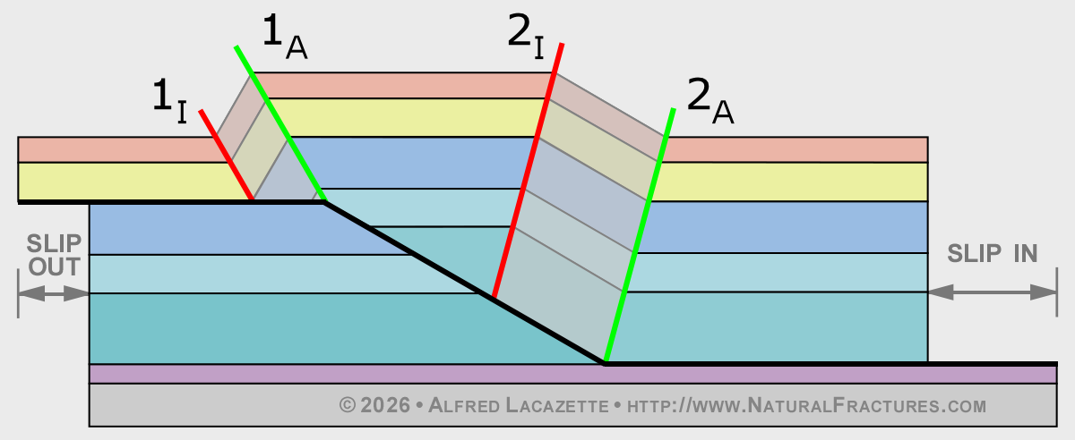
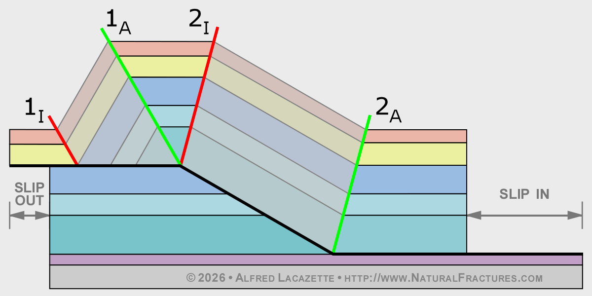
Inactive axial plane 2 has reached the top of the ramp. Most of the strata that overlie the ramp have been folded, but the triangle between axial planes 1A and 2I still has not been folded. Inactive axial planes (red) move with the hangingwall block.

Figure 4. End of anticlinal growth.

Anticlinal broadening stage

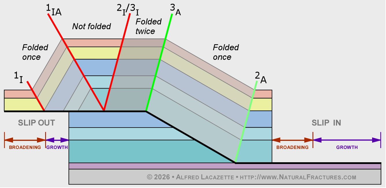
Active folding commences at the top of the ramp at axial plane 3A which forms when axial plane 2I is transported past the top of the ramp and out along the flat. Axial plane 1 becomes inactive when this happens. Folding at axial plane 3A refolds strata that were previously folded at axial plane 2A. The triangular area between axial planes 1 and 2 is never folded. Rocks forward (to the left in this case) of axial plane 3A are transported passively. Slip is not consumed by folding during anticlinal broadening, so the slip-rate is the same along the entire fault.

Figure 5. Anticlinal broadening stage.

Implications for reservoir geology

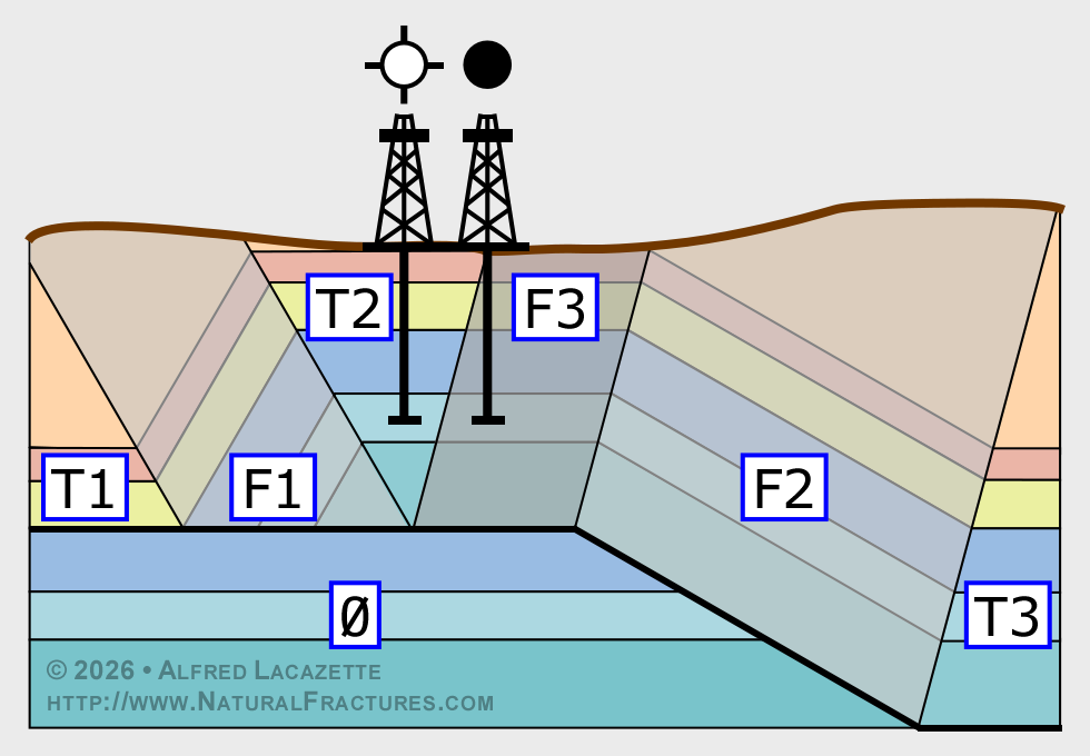
At least seven different structure/fracture domains are present in this simple, idealized cross-section. The top of this anticline is composed of two very different structural domains even though the structure and stratigraphy appear identical in maps and cross-sections. Fracturing of the forelimb and backlimb occurred under different conditions so that F2 and F1 may be very different geologically. This point is important because structural experts working in the oil industry normally do not differentiate domain T2 from F3 in maps and cross-sections because quantitative structural analysis is usually done only to define structural traps, not the flexure history of packages of rock.

In theory, T1, T2, and T3 are undeformed so that on average the types and density of fractures and other minor structures should be the same in each domain. In nature, T1, T2, and T3 were transported in different relative positions so each domain may have suffered some fracturing and each domain may have somewhat different fluid-transport properties. However, given that the packages were passively transported, they should be much less fractured than the other domains.

Fracturing and other reservoir-scale deformation features observed in outcrops may closely resemble reservoir rock deformation because structural domains can extend to the surface.

Figure 6. Structural domains in a fault-bend fold.

2D Example: Fault-bend fold in outcrop, Neuquen Basin, Argentina

Photograph showing the forelimb of a fault-bend fold in an outcrop of limestones and shales. The fold is in the early stages of anticlinal growth. Fractures are much more abundant in the folded panel (F1 in Figure 6). The fault began as a sharp break forming a planar ramp and flat joined at a sharp corner, as illustrated in Figures 1 through 7. The corner broke off and the fault progressively developed a damage zone with continued slip. The complex fault zone shape and several minor faults produced additional fractured and folded panels in the hangingwall block that are visible in the unannotated detailed photo below.

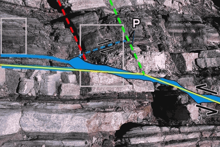
P: Pen for scale.   Solid yellow line: Original trace of fault.   Dashed green line: Active axial plane.   Dashed red line: Inactive axial plane.   Solid blue: Fault zone and fault strands.   Dashed blue line: Minor backthrust.   Half-arrows show the sense of motion across the faults.   Left-hand rectangle: Slightly fractured rocks in the never-folded but transported domains above the upper bedding-parallel fault segment (domain D6 in Figure 6).   Right-hand rectangle: Heavily fractured rocks in the once-folded domain above the fault (domain F1 in Figure 6).   Left rectangle: almost unfractured rocks in the never folded but transported domain (T1 in Figure 6).   Note that rock below the fault (domain 0 in Figure 6) are comparatively unfractured.

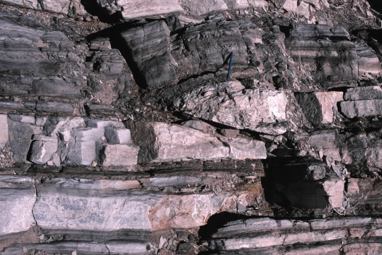
Figure 7. Fault-bend fold outcrop, Neuquen Basin, Argentina.

The third dimension

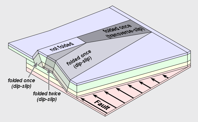
Figure 8 is a three-dimensional view of a fault-bend fold anticline. The plunging nose of the anticline results from decreasing displacement along the fault.

Each plunging nose has an additional structural domain that was folded by transverse flexural-slip, which is slip parallel to the fold axis and perpendicular to the transport direction.

Development of the plunging fold nose requires transverse extension of the folded rocks, which violates the constant bed-length constraint used in 2-D models. This extension is accommodated by fractures.

In theory, transverse flexural-slip can distribute the strain across the entire fold and this is sometimes observed. However, fractures are often concentrated in the plunging fold noses where the transverse extension is concentrated.

The amount of fold-axis parallel extension as estimated from quantitative structural analysis of seismic data provides a direct estimate of the fracture strain, but not of the fracture porosity.

The flat-lying rocks ahead of and behind the fold (as in Figure 6) have also been transversely extended due to the change in displacement along the fault and should be fractured.

Plunging fold noses also can form at lateral ramps, which are fault ramps that strike parallel to the transport direction. Regardless of the mechanism that causes fold closure, the strata in any fold with plunging noses must have been extended transversely to accommodate the increase in stratigraphic length required by the plunging fold noses.

Figure 8. 3D structural domains in a fault-bend fold.

3D Example: Nan Yi Shan field, Qaidam Basin, China

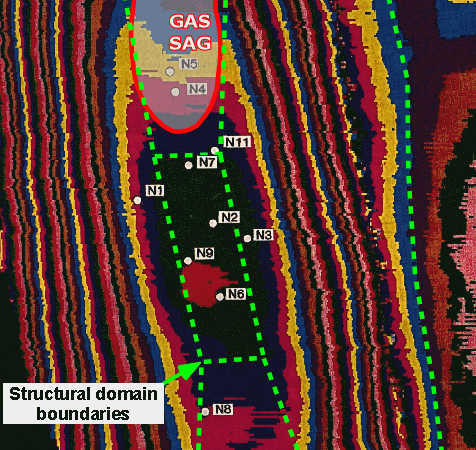
Time slice from 3D seismic survey across Nan Yi Shan field showing localization of gas sag on the northern plunge-panel of the fold. The best production test results from the fractured reservoir were from wells in the gas sag zone. Wells on the structurally higher fold crest had poorer tests. This suggests that localized fracturing in the plunge panel domain improved reservoir porosity and permeability.

After: R.J. Paul, 1993, Seismic detection of overpressuring and fracturing. An example from the Qaidam Basin, People's Republic of China, Geophysics, v.58, no. 10, p. 1532–1543.

Figure 9. Time slice from 3D seismic survey, Nan Yi Shan field, Qaidam Basin, China.

Fault propagation folding

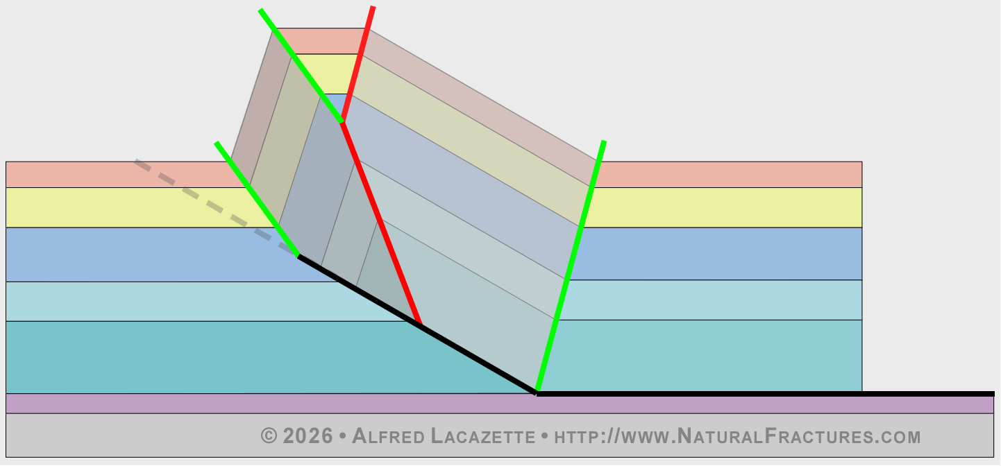
An illustration of constant bed thickness fault propagation folding is given below. The purpose of this section and the following section on trishear folding is simply to show that there are many possible geometries that develop during contractional folding. This page does not cover other contractional fold geometries such as area balanced cross sections.

More than one type of fault propagation folding occur. For details on fault propagation folding, read: Jon Mosar and John Suppe, 1992, BOOK CHAPTER - Role of shear in fault-propagation folding: in K.R. McClay, Thrust Tectonics, p.123-132.

In the figure below, the fault propagates incrementally, unlike the fault in the section on fault bend folding where the fault forms entirely prior to significant fault slip. The dashed gray line shows the future path of the fault. Note that folding consumes all the slip so that there is no slip out. There are two folded domains that are fractured (gray). The fault angle, bed dips, and axial plane angles can vary.

Trishear folding

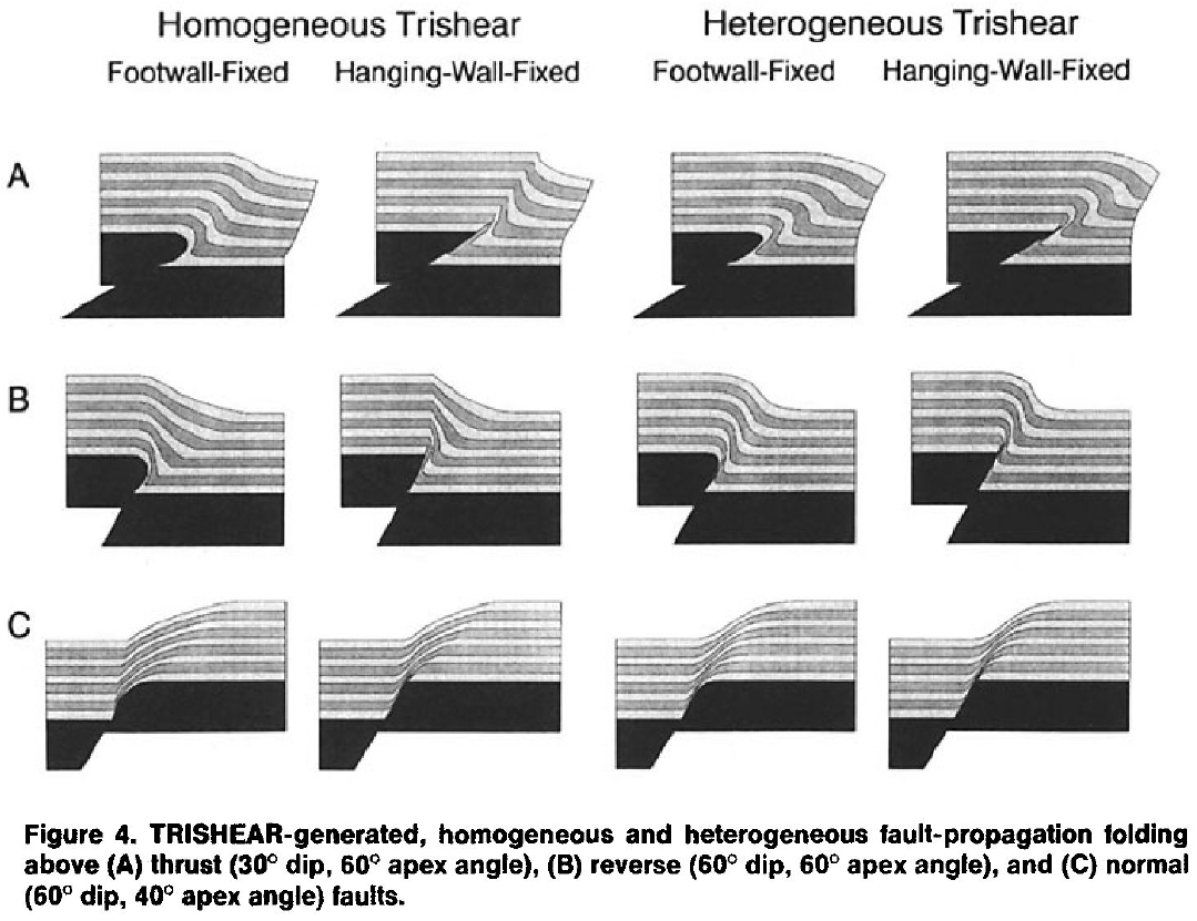
Eric Erslev wrote the original paper on trishear folding. The figure below is from that paper.

Trishear folding has been found to be broadly applicable to many contractional and extensional folds. Trishear explains curved bedding surfaces in folds, unlike the simple kink-band fold models described above on this page. Unlike fault-bend folding and fault-propagation folding, there is no analytical solution for the geometry of trishear folding. Instead, computer modeling is required. Detailed coverage of trishear folding is beyond the scope of this page, which is intended only to explain some basics and stimulate thinking on how fault-related folding localizes fractures. For a comprehensive discussion of trishear folding, read:

Stuart Hardy and Richard W. Allmendinger, 2011, Trishear: A Review of Kinematics, Mechanics, and Applications: in K. McClay, J. Shaw, and J. Suppe, eds., Thrust fault-related folding: AAPG Memoir 94, p. 95 – 119.

Figure 1. Figure 4 from Eric. A. Erslev, 1991, Trishear fault-propagation folding: Geology, v. 19, June, p. 617-620.